Signal processing

This notebook provides an overview of the functions provided by the elephant signal_processing module.

import neo
import numpy as np
import quantities as pq
import elephant
from elephant.signal_processing import *
from elephant.datasets import download_datasets
import matplotlib.pyplot as plt

All measures presented here require one or two neo.AnalogSignal objects as input. For this, we use an electrophysiology recording, and this data file contains one trial of an experiment.

# TODO: this is just for development and using local data, delete before merging
from pathlib import Path
filepath = Path('~/gin/elephant-data/tutorials/tutorial_signal_processing/data/i140703-001_single_trial.nix').expanduser()

# Download data
# repo_path='tutorials/tutorial_signal_processing/data/i140703-001_single_trial.nix'
# filepath=download_datasets(repo_path)

with neo.NixIO(f"{filepath}", 'ro') as file:
    block = file.read_block()

signals = block.segments[0].analogsignals[0]

1. Z-Score

The recordings from the different electrodes might have different offsets and amplitudes. So, it’s helpful for the later analysis to first z-score the signals. This way, all electrodes are normalized to a common range of values.

Here, we use the zscore function to normalize the signal. The inplace option is set to False to avoid overwriting the original signal, as it is required for subsequent examples.

signal = signals[:,1]

z_scored_signal = zscore(signal, inplace=False)

The result is the z-scored signal, as shown in the plots below.

# Plot the original signal
plt.figure(figsize=(10, 5))

# Plot the z-scored signal
plt.plot(z_scored_signal.times, z_scored_signal, label='Z-scored Signal', color='orange')

plt.xlabel(f'Time ({signal.times.dimensionality})')
plt.ylabel('Amplitude')
plt.title('Original Signal and Z-scored Signal')
plt.legend()
plt.xlim(signal.t_start, signal.t_start + 1*pq.s)

# Show the plot
plt.show()

2. Power Spectrum

Before delving into advanced methods, calculating and visualizing the power spectrum is a fundamental step in analyzing analog signals. Let’s compute and plot it for the first trial.

power_spectrum_f, power_spectrum_x = elephant.spectral.welch_psd(signals)
power_spectrum_x.shape

(96, 301)

Elephant is using the Welch algorithm to calculate the spectrum. It calculates the power spectra for all channels in the AnalogSignal object individually. For a better overview we can also look at the average power over all channels.

avg_power_spectrum_x = np.nanmean(power_spectrum_x, axis=0)

plt.semilogy(power_spectrum_f[:40], avg_power_spectrum_x[:40], color='orange')

plt.xlabel(f"frequency [{power_spectrum_f.dimensionality}]")
plt.ylabel(f"power [{power_spectrum_x.dimensionality}]");

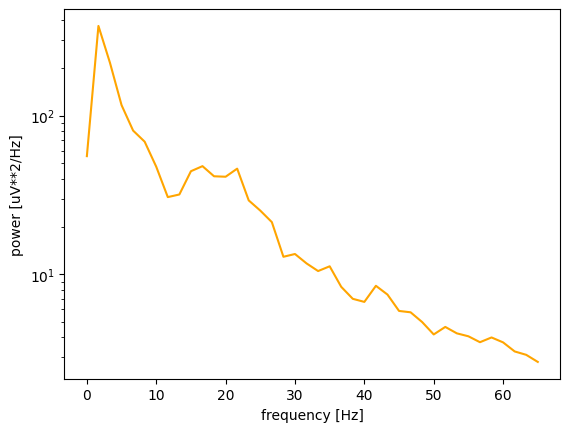
From the power spectrum we can guess the dominant frequencies: 10 - 30 Hz which corresponds to the Beta band.